Bench Matters

Middleware vendors offer moving averages modules for use as a quality assurance tool for the clinical laboratory. But what is a moving average? What does it offer the laboratory, and how would a laboratory set up moving averages?

Moving averages is a metric that monitors in real time the average patient value for any given analyte. A simple arithmetic moving average can be thought of as a moving window. Only results visible in the window are included in the mean calculation. With each new patient result the window moves by one patient result while the oldest value drops out of view. The mean is recalculated and data point plotted on a Levey-Jennings chart. In the absence of systematic error, the mean patient value doesn’t deviate significantly from the historic patient mean. A mean exceeding predefined control limits thus indicates the possible presence of a systematic error.

The key to establishing moving averages protocols is to determine three parameters: 1) The size of the error you wish to detect (control limits); 2) how many patient samples need to be averaged (N); and 3) which values to exclude from the mean calculation (truncation limits). In my lab, we chose the reference change value calculation to determine control limits, but other choices might be as valid. However, determining the other two options for moving averages protocols is more difficult.

Different strategies to determine the truncation limits and N exist, but many use computer modeling. This doesn’t mean laboratorians have to be statistics wizards or computer programmers to use moving averages. Thankfully, a nomogram useful to establishing moving averages without computer modeling has been published (Am J Clin Pathol 1984;81:492–9). A key piece of advice I learned from my own experience in using this particular nomogram—or any other method—is to set yourself up for success and undertake moving averages only if you have patient results spanning several calibrations and assay lot number changes.

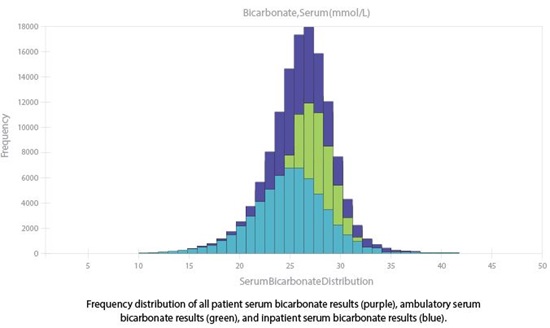
In our lab, we used this nomogram to establish moving averages protocols, which we subsequently tested via computer modeling. We used as our performance metric the average number of affected patient samples prior to error detection (ANPed) (Am J Clin Pathol 2000;113:240–8). We found our systematic error detection was acceptable for a number of assays. For example, with an ANPed of 46 we detected a positive error of 4 mmol/L in the mean bicarbonate concentration. However, we found that assays with skewed distributions hinder detection of systematic error. For instance, serum bicarbonate has a slight negative skew (Figure 1, purple curve), and consequently we detected a negative 4 mmol/L error with an ANPed of 111.

Placement of truncation limits largely accounts for the difference in ANPed within the same protocol. If the distribution is Gaussian, or nearly so, truncation limits placed outside of the patient distribution can be varied with essentially no change in ANPed. In skewed distributions, samples further away from the central distribution have disproportionate influence and need to be truncated out. The challenge is selecting where to place the truncation limits. For bicarbonate, changing the lower truncation limit by just 1 mmol/L—from 20 mmol/L to 19 mmol/L—changed the ANPed from 111 to 74 samples.

So how can we monitor skewed distributions? In our lab, we noted that for some analytes the skew was due partially to the difference between ambulatory and inpatient distributions (Figure 1) and since the two populations are typically measured at different times of the day, we developed protocols for each sub-population. Using this strategy, a negative 4 mmol/L error for bicarbonate in the ambulatory population would be detected with an ANPed of 58. Although splitting the population does have downfalls by reducing the number of samples tested, in the absence of computer modeling this strategy can reduce ANPed. However, for significantly skewed distributions other methods of determining N and truncation limits are needed; in our case, this meant computer modeling.

Modeling enabled us to produce protocols for analytes with skewed distributions by randomly varying N and truncation limits to find ideal parameters. This included a protocol for creatinine that detects a positive systematic error of 0.30 mg/dL with an ANPed of 55 samples. Modeling is challenging and time consuming, but if you can do it, or arm-twist someone who can into helping you, the rewards are great.

Ultimately the challenges in setting up moving averages are worth the rewards. Appropriately established moving averages protocols can detect a systematic shift hours before your next QC event, a goal well worth the effort.